It Feela Like Stomach Acid Is Burning My Throa

: Percentages

This publication will present the following question:

*

How to calculate percentages in Excel?

*

"A percentage is a way to represent how much an amount in respect of another (the reference)." 1

The importance of this issue, if it is not what formula would you use?, because once you know the math normal use ( sum , subtraction, multiplication and division), calculate a percentage is laughable, the reality is that the percentages can be done with a simple division .

Central to this publication is to understand how we can calculate a percentage in different forms and variations mathematics, especially given the essence of our blog, know how we can perform in Excel.

Our entry will be divided into:

• Calculate the percentage of an amount in Excel
• obtaining a share of Excel
  proportion

CALCULATE PERCENTAGE OF AMOUNT IN EXCEL

*

The calculation of a percentage of a quantity, in other words, illustrating with an absolute value ( 1000 in this example ) means

1000 That represents 100 % a value, ie the total value and / or absolute amount.

If you would like to know which is 10% 1000, would run some of the following:

Procedure 1

Math : 10 * 1000 / 100

Excel Procedure:

a) Write the cell where you want the result, the sign = (
b) Add the percentage number. In this example is 10
c) The next step to add the sign * (asterisk). This will apply a multiplication .
d) Add the absolute number, ie the total value. This example is the 1000
e) Once the value added total formula to close the parenthesis ) .
f) Now add parentheses after the sign / (diagonal). Apply to this division.
g) Now add the 100 . This value is always fixed, never varied in comparison 10 (percentage) and 1000 (total, accounting for 100 % percentage.
h) Press ENTER or OK.
The formula would be as follows: = (10 * 1000) / 100

The result in this case is 100. The number 100 represents 10% 1000.

Procedure 2

Math: % 1000 * 10

Excel Procedure:

a) Write the cell where we want the result, the sign =
b) Add the number or value of our total or absolute amount. In this case 1000.
c) after the number now add the sign * (asterisk). This will apply a multiplication .
d) Add the number percentage. In this example is 10 %
e) Press ENTER or OK.
The formula would be as follows: = 1000 * 10 %

The result in this case is 100. The number 100 represents 10% 1000.

Procedure 3

continue with the example of calculating the 10 % of 1000 but now applying the % indirectly. This in other words, means that no multiply by 10 %, but by 0.10 . The 0.10 is the same as if calculated by 10 % , as this represents the first tenths of 10 % (10/100 = 0.10). The procedure is as follows:

Math : 1000 * 0.10

Excel Procedure:

a) Write the cell where you want the result, the sign b =
) Add the number or value of our total or absolute amount. In this case 1000.
c) after the number now add the sign * (asterisk). This will apply a multiplication .
d) Add the number percentage. In this example is 0.10 (10 / 100 = 0.10) .
e) Press ENTER or OK.
The formula would be as follows: = 1000 * 0.10

The result in this case is 100. The number 100 represents the 0.10 (10 %) of 1000.

*

*

PROCUREMENT PERCENTAGE OF RELEVANT TO SHARE

is common that you need to know the counterpart of calculating a percentage of a quantity, that is, you need to know that it represents X amount over another, proportional to the total value or all.

To explain this issue will continue with the example of the number 1000 the total value and / or absolute. If you would like to know what percentage represents 200 the absolute amount in this case is 1000 , you would run some of the following:

Procedure 1

Math: 200 / 1000 * 100

Procedure in Excel obtaining the percentage as an integer value :

a) Write in the cell where you want the result, the sign = (
b) Add the number proportionately. In this example is 200 .
c) The next step is to add the sign / (diagonal). This will apply a division .
d) Add absolute number, ie the total value. This example is the 1000 .
e) Once the total value added end the formula with a break ) .
f) Now add the numbers after * (asterisk). This will apply a multiplication .
g) Now add the 100 . This value is always fixed, never varied in comparison of 200 (value share) and 1000 (total), accounting for 100% of the percentage.
h) Press ENTER or OK.

formula would be as follows: = (200 / 1000) * 100

The result in this case is 20. The number 20 represents 20% 1000. Excel for this operation, we only threw 20 as an integer value and not a strictly text "20 % ." Logically understood that 20 is equal to 20% (200) 1000.

Procedure 2

Math: 200/1000

Excel Procedure to obtain a percentage percentage (sic):

a) Write the cell where you want the result, the sign =
b) Add the number proportionately. In this example is 200 .
c) The next step is to add the sign / (diagonal). Apply to this division.
d) Add the absolute number, ie the total value. This example is the 1000 .
e) Press ENTER or OK.

The formula would be as follows: = 200 / 1000

The result in this case is 0.2 or 0.20.

order to convert the 0.2 to rate one must choose the format bar option percentage.



Sources:

1 http://thales.cica.es/rd/Recursos/rd99/ed99-0249-04/apartado41 . htm
http://maralboran.org/wikipedia/index.php/Porcentajes


Posted by: Julio Rosales V.

Culo De Jenifer Lopez

Excel XLS: XLS

In this paper I shall answer the following questions:

How to calculate power or an exponential number in Excel?

To "raise" a number of specific power, I propose two methods:

• simple formula
• function formula

Formula simple:

Suppose you want to "raise" the number 2 to the fifth (5th) power this mathematically would multiply the number 2 , by itself, 5 times. The math looks like this: 2 * 2 = 4 * 2 = 8 * 2 = 16 * 2 = 32. Note

you that number 2 is multiplied by itself initially, and then by the result and multiply to 5 times.

This simple math we can do it in Excel. The Formula
would be as follows:

= 2 * 2 * 2 * 2 * 2

If you notice carefully analyzes the formula is simple. But now suppose a more severe case where you want the number 2 raised to the hundredth power. That means I would have multiply the 2 by itself 100 times. The former method would be a good solution only for people with great patience and above all a long time.

Instead I propose a much simpler solution:

The process is as follows:

a) Write the cell where you want the result, the sign =
b) Add the number or value potentiate want.
c) after the number now add the sign ^ (caret (colloquially known as the roof, outbuilding or umbrella). This sign we get it through your keyboard, pressing ALT + 94 (Press ALT-straight-without letting go and write 94, then release ALT and get the sign ^ ).
d) Add after the caret (^ ) the number which will be lifted. The formula could be as follows: = 2 ^ 100

e) Press ENTER or OK.

press the OK result might look like:

Perhaps the result seems wrong or solve a number incomprensible.Para this case, one must go:

a) Menu Format
b) Sub Cells
c) Choose the Number tab
d) In the Categories list select the option again number and accept.

With these final steps in his cell the result should resemble the one shown in the red box below the image.

function formula:

Exactly the same process as we can to "raise" the number 2 to the fifth (5th) we can achieve power by an Excel function. Function Power is . The structure of the function is POWER (number, power) .

The process is as follows:

Following the example of the number 2 raised to the hundredth power formula would be as follows: = POWER (2, 100) . The procedure is as follows.

a) Write the cell where you want the result, the sign = POWER (
b) Add the number or value that you want to potentiate.
c) Add immediately after the number to enhance the sign ;
d) Now add the power number, ie, the number to which you wish to raise.

a) After adding the power function with a closing parenthesis ) and now you can press ENTER or OK.

press the OK result might look like:



Again, I repeat, if the result as in the "formula with circumflex" seems wrong or incomprehensible numbers may resolve this by following the steps mentioned above:

a) Menu Format
b) Sub Cells
c) Choose the Number tab
d) In the Categories list select the option again number and OK.

With these final steps in his cell the result should resemble the one shown in the red box below the image.







** The equivalent function POWER in English is POWER.
** Remember the = sign should always go to top of any formula. **
If your computer is configured in the English language, you may need to use: instead of; This observation stress for those who prefer to manually write the complete formula instead of using the cursor or mouse when choose to join the ranks. **
Excel only operate only with numeric values: integers, decimal, date, time, etc. but NEVER TEXT type characters .
** Remember that the wording of the formulas should never have spaces between one character to another.


Posted by: Julio Rosales V.

Best Shoulder Protector Beginning Rugby

Powers in Excel: Subtract, Multiply and Divide in Excel XLS

In this paper I shall answer the following questions:

subtract in Excel How? What is the function used in subtraction?

How to multiply in Excel? What use in a multiplication function?

How to split in Excel? What role use in a division?

arithmetic

These three have something in common and this similarity is that NO function in Excel to divide and subtract, multiply omitted.

However, if there is certainly ways to do such operations in Excel . In addition to the procedural default menu Insert> Function , you can do " with simple formulas " .

then expose the 2 procedures so you can make these calculations in Excel :


1 .- OPERATION WITH FIXED VALUES IN A CELL

As the procedure is the same for subtraction, multiplication and division using arithmetic symbols, then I take the liberty to expose the three operations simultaneously .

The process is as follows:

a) Write the cell where you want the result, the sign =
b) Add the number or value that you want to subtract, multiply or divide, which must be strictly numeric.
c) After adding the value, add the sign - (hyphen for subtraction), / (diagonal to divide) and * (asterisk for multiplication), this will depend on the extent of the operation that seeks to make. These signs can easily find at the top of its keypad.

order to add more than one value repeat step B and C. You can add as many numbers as you want and how its operation is permitted, as the example in the formula bar (see image below).

d) Once the values \u200b\u200bentered the function with a closing parenthesis ) and now you can press ENTER or OK.


This method is too crude. Is recommended only for small transactions when cell values \u200b\u200bare fixed.

The formula could be in the following ways:

** Remember that the sign = should always be at the beginning of any formula. **
Excel only performs mathematical operations on numeric values: integers, decimal, date, time, etc. but NEVER TEXT type characters .



2 .- OPERATIONS DIFFERENT VALUES IN CELLS WITH FIXED OR VARIABLE

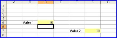
There are situations where the operation of the cells are values \u200b\u200bthat are in different positions, distant from each other, either by columns or rows (see image-example).

There are also occasions where the values \u200b\u200binserted into a cell are constantly being updated or modified. This example is unusual in payment formats, payroll or any format to serve literally as a calculator (see image-example).

The process is as follows:

a) Write in the cell where you want the result, signs = (
b) Add the number or value that you want to add by selecting with your mouse or cursor cell where the first value.
c) After adding the value add the sign - (hyphen for subtraction), / (diagonal to divide) and * (asterisk for multiplication), this will depend on the extent operation that seeks to make.

order to add more than one value repeat step B and C. You can add as many numbers as you want and how its operation is permitted, as the example in the formula bar (see image below).

d) Once selected cells function with a closing parenthesis ) and now you can press ENTER or OK.


Our example was as follows:

productive roles (Multiply )

Continuing with the previous year, the procedure is as follows: The

structure function is: = PRODUCT (number1, number2, issue3 ,...)

The procedure is as follows:

a) Writing in the cell where you want the result, the sign = PRODUCT (

b) Add the number or value that you want to multiply. This can write it manually or you can select the cell where the value is. In this case, select cell B3 and then B5.

c) Remember to go Sepra each number or value of selected cell with the sign , or ; , so depending on the configuration on your keyboard.

d) Close function with a break ) and now you can press ENTER or OK.

= PRODUCT (B3, B5)

Posted by: Julio Rosales V.